[Statistics] GWR vs OLS

Paper Review : Spatial Regression and Correlation

date : 2022.12.09

presenter : Woojeong Park

---

목표

• OLS, GWR 이해
• 각각의 장점 및 단점
• statistics

---

OLS

OLS 개념

• Ordinary Least Squares, 전통적 회귀분석으로 여겨짐
• observations 간의 독립성과 오차 동분산성(homoscedasticity)를 가정
  • 표집 위치에 상관없이 관찰들은 서로 독립적이어야 하고, 종속변수의 관찰값과 추정값의 차이인 오차(errors)가 상호 독립적이며 분산이 일정한 것으로 가정한다.
  • 공간적으로 근접한 위치에 표집 된 사례일수록 유사한 값을 가지는 경향이 있기 때문에 현실적으로 이러한 가정이 충족되기는 어려움

---

OLS mathematical background

\(\begin{align*} y_i = \beta_0 + \sum_{j=1}^p X_{ij} \beta_j + \epsilon_i \end{align*}\) Where \(\begin{align*} \beta_0 &= \text{ Intercept coefficient}\\ \beta_j &= \text{ Solpe Coefficient for the $j$th independent variable $X_j$} \\ \epsilon_i &= \text{ Random error term with N(0, $\sigma^2I$)} \\ I &= n \times n \text{ identity matrix} \end{align*}\) —

OLS mathematical background

In the matrix notation \(Y = X \beta + \epsilon\)

The least square estimate of $\beta$ is \(\hat{\beta} = (X^T X)^{-1} X^T y\) —

OLS mathematical background

ANOVA can be performed to check whether the regression model is statistically significant or not(F-value and corresponding p-value).

T-test(p-value) for eaach parameter estimates can be perforemd to see whether they are statistically significant or not.

\[T = \frac{\hat{\beta}}{s / \sqrt{s_{xx}}}\]

Where \(\begin{align*} \hat{\beta} &= \frac{s_{xy}}{s_{xx}} \\ s_{xy} &= \sum (x-\bar{x})(y-\bar{y}) \\ s_{xx} &= \sum (x-\bar{x})^2 \end{align*}\) —

OLS mathematical background

Coefficient of determination can be calculated to see how well the model is successful at explaining variability as \(R^2 = \frac{S_{xy}^2}{S_{xx}S_{yy}}\)

---

OLS mathematical background

To check normality assumption, Shairo-Wilk test can be performed \(W = \frac{\left( \sum_{i=1}^n a_i x_{(i)} \right)^2}{\sum_{i=1}^n (x_i - \bar{x})^2}\) Where \(\begin{align*} x_{(i)} &= \text{ Ordered sample values($x_{(1)}$ is the smallest)} \\ a_i &= \text{ constants generated from the means, variances and covariances of the order statistics of a sample of size $n$ from a normal distribution.} \end{align*}\)

Shairo-Wilk test tests the null hypothesis that a sample $x_1, \cdots, x_n$ came from a normally distributed population. The test rejects the null hypothesis if $W$ is too small.

• 귀무가설 : residual은 정규분포와 같다.

  또다른 normality assumption test 방안

  Jarque-Bera test can be also performed for testing the normality assumption. \(JB = \frac{n}{6} \left( S^2 + \frac{K^2}{4}\right)\) Where \(\begin{align*} S &= \text{Skewness} \\ K &= \text{Kurtosis} \\ n &= \text{number of observations} \end{align*}\)

이는 카이제곱분포를 따르고, 위의 경우과 같은 귀무가설을 테스트한다.

---

공간적 등분산성 검정

The Breusch-Pagan test on random coefficients and White test on specification robust can be performed to check the presence of spatial heteroscedasticity (i.e. spatial non-stationarity).

---

공간적 등분산성 검정 : Breusch-Pagan Test

• Breusch-Pagan Test : whether the estimated variance of the residuals from a regression depend on the values of the independent variables or not.
• \[\begin{align*} \text{regression : } Y_i = \alpha + \beta X_i + \epsilon_i \\ \text{auxiliary regression : } Z_i^2 = \phi + \delta X_i + \nu_i \end{align*}\]

Where \(\begin{align*} &i \in \{1, 2,\cdots, N\} \\ &\mathbb{E}(\epsilon_i) = 0 \\ &S^2 = \sum \hat{u_i}^2 / N \\ &Z_i^2 = \sum \hat{u_i}^2 / S^2 \\ &\hat{u_i} = \text{residuals} \end{align*}\) —

공간적 등분산성 검정 : Breusch-Pagan Test

• Step 1 : Apply OLS in the model
• Step 2 : Compute the regression residuals ${\displaystyle {\hat {u}}_{i}}^2$ and divide by the Maximum Likelihood estimate of the error variance from the Step 1 regression to obtain $S^2, Z_i^2$
• Step 3 : Estimate the auxiliary regression(여기서의 $X_i$는 origin regression의 $X_i$와 달라도 됨)
• Step 4 : 검정통계량 $LM$ 계산 \(LM = \frac{1}{2} (TSS - TRR)\) Where where TSS is the sum of squared deviations of the $Z_i^2$ from their mean of 1, and SSR is the sum of squared residuals from the auxiliary regression.

---

공간적 등분산성 검정 : Breusch-Pagan Test

검정통계량은 freedom = $p-1$인 $\chi^2$ 분포를 따른다.($p$ is the number of estimated parameters in the auxiliary regression.) \(LM = \frac{1}{2} (TSS - TRR) \sim {\displaystyle \chi _{p-1}^{2}}\)

---

공간적 등분산성 검정 : Breusch-Pagan Test

The testable hypothesis are expressed as follows: \(\begin{align*} &H_0 : \delta = 0 \text{ (homoscedastic error variance)} \\ &H_a : \delta \neq 0 \text{ (homoscedastic error variance)} \end{align*}\)

• If the test statistic has a p-value below an appropriate threshold (e.g. p < 0.05) then the null hypothesis of homoskedasticity is rejected and heteroskedasticity assumed.
• $\delta=0$이면, 즉 귀무가설 성립 시 empirical error variance는 상수텀이고, 대립가설이 참이면 empirical error variance는 $X$ variable에 대한 함수라고 해석할 수 있다.

---

공간적 등분산성 검정 : White Test

• Breusch-Pagan : detect only linear forms of heteroskedasticity
• White : The residuals are computed from the original model and an empirical measure for the error variances is constructed by squaring them. \(\begin{align*} &\text{regression : }Y_i = \alpha + \beta_i X + \beta_2 W + \epsilon_i \\ &\text{auxiliary regression : } \hat{u_i}^2 = \phi + \delta_1 X_i + \delta_2 W_i + \delta_3 X_2 + \delta_4 W_2 + \delta_5 X_i \times W_i + \nu_i \end{align*}\)
• 검정통계량은 Lagrange multiplier (LM) test statistic을 이용(단, $p$ is the number of estimated parameters in the auxiliary regression.) \(LM = n R^2 \sim {\displaystyle \chi _{p-1}^{2}}\) —

  공간적 등분산성 검정 : White Test

• Step 1 : the squared residuals from the original model serve as a proxy for the variance of the error term at each observation.(residual ~ normality 가정)
• Step 2 : The independent variables in the auxiliary regression account for the possibility that the error variance depends on the values of the original regressors in some way (linear or quadratic)
• Step 3 : If the error term in the original model is in fact homoskedastic (has a constant variance) then the coefficients in the auxiliary regression (besides the constant) should be statistically indistinguishable from zero and the R2 should be “small”.

---

공간적 등분산성 검정 : White Test

The testable hypotheses are expressed as follows: \(\begin{align*} H_0 : \delta = 0 \text{ (homoscedastic error variance)} \\ H_a : \delta \neq 0 \text{ (homoscedastic error variance)} \end{align*}\) White test는 등분산성, 이분산성 하에서 least square estimator의 표본분산을 비교한다. 귀무가설이 참이라면, variance에서 발생하는 차이들은 sampling에 의한 오차이지, 근본적 차이에 의한 오차가 아니라고 볼 수 있다.

---

GWR

GWR 개념

• GWR is an extended version of traditional OLS regression

• global만 집중하는 OLS에 비해 local reality 반영 위해 GWR 사용

  GWR mathematical background

  회귀식은 아래와 같이 표현가능하다.

\(y_i(\mu) = \beta_{0i}(\mu) + \beta_{1i}(\mu)x_{1i}+ \cdots + \beta_{mi}(\mu)x_{mi} + \epsilon_i(\mu)\)

• $\mu$ : 위치
• $y$ : 종속변수
• $m$ : 독립변수 $x$의 개수
• $\beta$ : 회귀계수
• $\epsilon$ : 오차항

• $i \in {1, 2, \cdots, n }$ : 관측 인덱스

  GWR mathematical background

  위치정보 $\mu = (u_i, v_i)$ : set of location co-ordinates of $i$-th point over space. 를 반영하여 다시 쓰면

\(y_i = \beta_0 (u_i, v_i) + \sum_{j=1}^p X_{ij}\beta_j (u_i, v_i) + \epsilon_i\) Where \(\begin{align*} \beta_k(u_i, v_i) &= \text{ Continuous function of the location $(u_i, v_i)$ at point $i$} \\ \epsilon_i &= \text{ Random error term with $N(0, \sigma^2 I)$} \end{align*}\)

In matrix notation, \(Y = \beta \bigotimes X + \epsilon\) Where $\bigotimes$ means componentwise-multiplication.

---

GWR mathematical background

The matrix $\beta$ consists of $n$ sets of local parameters, which is given as \(\beta = \begin{bmatrix} \beta_0 (u_1, v_1) & \beta_1(u_1, v_1) & \cdots & \beta_k (u_1, v_1) \\ \beta_0 (u_2, v_2) & \beta_1(u_2, v_2) & \cdots & \beta_k (u_2, v_2) \\ \cdots & \cdots & \cdots & \cdots \\ \beta_0 (u_n, v_n) & \beta_1(u_n, v_n) & \cdots & \beta_k (u_n, v_n) \\ \end{bmatrix}\)

---

GWR mathematical background

여기서 가중 최소자승법(Weighted Least Square Estimation)을 이용하자.

즉, $\mu=(u_i, v_i)$에 대하여 \(\epsilon(\mu) = y_i(\mu) - \beta_{0i}(\mu) + \beta_{1i}(\mu)x_{1i}+ \cdots + \beta_{mi}(\mu)x_{mi}\) 에 대하여 weight $W_i$를 생각하자.공간가중행렬 $W_i$는 $i$번째 관측값과 다른 모든 관측값을 반영하는 공간행렬로, $i$번째 관측값의 거리에 기초한 가중치 $d_i$를 포함하는 $n \times n$ 대각행렬이다.

\(W_i = \begin{bmatrix} w_{i1} & 0 & 0 & \cdots & 0 \\ 0 & w_{i2} & 0 & \cdots & 0 \\ \vdots & \vdots & \vdots & \cdots & \vdots \\ 0 & 0 & 0 & \cdots & w_{in} \\ \end{bmatrix}\) —

GWR mathematical background

\(\underset{\beta_{ij}, i \in \{1, \cdots,n \}, j\in\{1,\cdots,m\}}{\text{minimize }} \sum_{i=1}^m W_i \{\epsilon_i(\mu)\}^2\) 이를 달성하면 된다. 이는 각 $\beta_{ij}$에 대하여 미분하여 solution을 구하면 다음과 같이 표현된다. \(\begin{align*} \hat{\beta}_i = (\hat{\beta_{i0}},\hat{\beta_{i1}},\cdots,\hat{\beta_{im}})^T = (X^T W_i X)^{-1} (X^T W_i Y) \end{align*}\)

적당한 matrix calculation을 통해 다음을 얻는다.

\[(X^TWX) \hat{\beta} = X^T W Y\]

따라서 최종적인 회귀계수 추정식은 아래와 같이 얻어진다. \(\hat{\beta} = [X^TWX]^{-1} X^T W Y\) —

kernel selection

커널함수는 가중치를 만드는 대역폭이 고정되어 있는 고정방식(Fixed spatial kernel), 그리고 관측치 수에 따라 다른 대역폭을 사용하는 가변방식(adaptive spatial kernel) 이 있다. 주로 관측치가 조사지역에 규칙적으로 있으면 전자, 관측치 분포가 다양하면 후자를 쓴다. 확실치 않은 경우, 후자가 안전하다.

가중치행렬 $W$는 여러 커널함수중에 하나를 택할 수 있는데, 주로 Gaussian form을 많이 쓴다. \(\begin{align*} &w_i(\mu) = \exp (-\frac{1}{2} \left(\frac{d_i(\mu)}{h}\right)^2) \\ &w_i(\mu) \text{ : 공간좌표에서 관측치 $i$에 대한 가중치} \\ &d_i(\mu) : \text{ : 관측치 $i$와 공간좌표 $\mu$간의 거리} \\ &h \text{ : 대역폭} \end{align*}\) —

kernel selection : bandwidth $h$

이 값은 대역폭 $h$가 커질수록 동일한 거리에 대한 가중치가 1로 계산되고, 이 경우 OLS와 같은 결과를 지닌다. 반면, 대역폭이 작아지면 가중치는 0으로 계산될 것이다.

GWR의 대역폭은 smoothing function 기능을 한다.

• high bandwidth : over-smoothed model, producing parameters with too little vairation across space

• low bandwidth : under-smoothed model, greater variation in model parameters over space than what is realistic.

대역폭 $h$의 선택

적정 대역폭 설정하기 위해서 AIC(Akaike Information Criterion) 또는 CV(Cross Validation) 가 사용된다. 관찰값과 추정값의 차이 및 모형의 복합성을 고려하는 AIC가 더 많이 선호된다.

bandwidth value의 선택방법은 3가지가 존재한다.

---

대역폭 $h$의 선택 1

First : selected based on existing knowledge. With a very large data set, bandwidth selection can be made using the desired percentage of the sample points to save time or otherwise can used all data.

---

대역폭 $h$의 선택 2

The second method of bandwidth selection in GWR requires no prior knowledge, and estimates bandwidth through a cross-validation technique which minimizes the squared error as \(z = \sum_i [y_i - y_{\neq 1}(h)]^2\) Where \(y_{\neq 1}(h) = \text{ Fitted value of $y_i$ with observation for location i omitted from the estimation process}\) This technique is only possible when the regression point locations are the same as the data point locations.

---

대역폭 $h$의 선택 3

The third method for bandwidth selection in GWR employs a technique which minimizes Akaike Information Criterion (AIC) for fitting the best regression model as \(AIC_c = 2n \log_e(\hat{\sigma}) + n \log_e(2 \pi) + n \times \frac{n+tr(S)}{n-2-tr(S)}\) Where \(\begin{align*} &n = \text{Sample size} \\ &\hat{\sigma} = \text{Estimated standard deviation of the error term} \\ &c = \text{subscript for corrected AIC estimate} \end{align*}\)

• lower AIC : reality에 가까운 model

---

Auto Correlation

• 과거과 미래에 영향을 주는 정도

Auto Correlation 측정법

• 측정법 : Moran I statistics 잔차의 공간적 자기상관성 측정 위해 가장 많이 쓰이는 지표

\(I = \frac{n \sum_{i=1}^n \sum_{j=1}^n w_{ij} (y_i-\bar{y})(y_j-\bar{y})}{\sum_{i=1}^n \sum_{j=1}^n w_{ij} \times \sum_{i=1}^n (y_i-\bar{y})^2}\)

• $n$ : 지역단위 수
• $\bar{y}$ : 종속변수 $y$의 평균
• $w_{ij}$ : $(i,j)$ 지점의 공간가중행렬

Moran I 지수 지역간의 인접성을 나타내는 공간가중행렬과 인접하는 지역들 간의 속성데이터 유사성을 측정하는 것!

---

Auto Correlation 측정법 : Moran I 해석

Similarity between observations for a given variables as a function of spatial distance가 측정된다. \(I = \frac{\sum_i^n \sum_j^n W_{ij} (y_i-\bar{y})(y_j-\bar{y})}{S^2 \sum_i^n \sum_j^n W_{ij}}\)

• $I>0$ : 특정 거리만큼 떨어진 observation들이 비슷하다고 여겨질 때 나옴
• $I<0$ : 특정 거리만큼 떨어진 observation들이 비슷하지 않다고 여겨질 때 나옴

• $I=0$ : 랜덤하게 + 독립적으로 관측값들이 뿌려져 있음

  Auto Correlation 측정법 : Moran I

  $I$를 통해서 검정통계량 $Z$ 생성가능 \(Z = \frac{I - \mathbb{E}[I]}{S_\epsilon (I)}\)

• $\mathbb{E}[I], S_\epsilon(I)$ : 통계량 $I$의 평균과 표준편차
• $Z=1$이다 == 유사한 값 가진 지역들이 인접하는 경향이 강함
• $Z=-1$이다 == 큰 값과 작은값 가진 지역들이 골고루 인접함
• 이렇듯, 큰 값들과 작은 값들이 공간적으로 밀집해 있는 경우 모두 동일하게 자기상관도가 크게 산출된다.

---

Auto Correlation 측정법 : Moran I

Moran I 지수의 통계적 유의성 검정을 통해 공간적 자기상관을 판정하여 공간적 자기상관이 존재한다면 지리가중회귀분석(GWR)으로 모형을 추정한다.

공간적 자기상관이 없는 것으로 판정되면 단순회귀분석(OLS)으로 모형을 추정하는 것이 가능하다.

---

Spatial Autoregression

Autocorrelation를 regression modelling process에 추가하여 spatial autoregression을 고려해보자. 이는

• additional regressor in the form of spatially lagged dependent variable
• error structure 들을 추가하여 구현가능하다. \(y = \rho Wy + X\beta + \epsilon_i\) Where \(\begin{align*} &y = \text{$n$ by 1 vector of observations on the dependent variable} \\ &W = \text{$n$ by $n$ spatial weights matrix that formalizes} \\ &\rho = \text{spatial autoregressive parameter} \\ &X = \text{$n$ by $k$ matrix of observations on the exgenous variables with an associated $k$ by 1 regression coefficient vector $\beta$} \\ &\epsilon = \text{a vector or random error terms} \end{align*}\) —

  Spatial Autoregression

  The log-likelihood for the spatial autoregression can be estimated by \(\ln L = -\frac{1}{2 \sigma^2} (y-\rho Wy-X\beta)^T(y- \rho Wy - X\beta)\) The least square estimator and variance for spatial autoregression can be estimated by \(\begin{align*} &\hat{\beta}_{ML} = (X^TX)^{-1} X^T (y-\lambda Wy) \\ &\hat{\sigma}_{ML} = (e_o - \rho e_L)^T(e_o - \rho e_L)/N \end{align*}\) Where \(\begin{align*} e_o = y-X\hat{\beta}_o \\ e_L = y-X\hat{\beta}_L \end{align*}\) —

Spatial Autoregression

• Spatial autoregression model을 위해서 Likelihood Ratio Test 가 시행될 수 있다.
• which corresponds to twice the difference between the log likelihood in this model and the log- likelihood in the standard regression model with the same independent variables with l equaling zero.
• 이는 $\chi^2_1$ distributed with one degree of freedom으로 시행된다.

---

Spatial autoregression 관찰

Spatial autoregression를 보기 위해 Lagrange Multiplier-Lag statistics 와 Robust Lagrange Multiplier-Lag statistics 를 생각해볼 수 있다.

\(LM_{Lag} = \frac{(e^TWy / s^2)^2}{(WX\beta^T)M(WX\beta) / s^2 + tr(W^TW + W^2)}\) Where \(\begin{align*} &M = I - X(X^TX)^{-1}X' \\ &y = \text{vector containing the dependent variable} \\ &e = \text{vector of OLS residuals} \\ &W = \text{spatial weights matrix} \\ &s^2 = e^Te / N \text{(ML estimate for residual variance)}\\ &\beta = \text{vector of OLS estimates} \end{align*}\) The Lagrange Multiplier lag Test($LM_{Lag}$)는 $\chi^2_1$ distribution을 갖는다.

---

Spatial Autoregression(SAR) : OLS의 한계

• Spatial autocorrelation : 가까이 위치한 관측치들의 lack of independence
• OLS는 관측치들의 independence를 가정하기 때문에 the presence of spatial autocorrelation in a dataset is troublesome for OLS regression
• This premise has been the foundation for a new regression technique called geographically weighted regression (GWR) to capture both spatial dependency and spatial non-stationarity in the modeling process.

• ---

  non-stationarity test

  The aim of a non-stationarity test is to examine whether the local variations as generated by GWR are significantly different over space.(차이가 있어야 GWR 사용한 것이 의미가 있음.)

• 원래는 time series analysis에서 사용되는 것
• 시간(공간)이 변해도 분포가 일정한가?에 대한 test
  • stationarity test : 시간(공간)이 변해도 분포 일정
  • Non-stationarity test : 시간(공간)이 변해도 분포 일정 X

---

non-stationarity test 1

• First method : comparing the range of the local parameter estimates with a confidence interval around the OLS estimate of the equivalent parameter.
  • The parameter is considered to be nonstationary if the interquartile range of GWR estimates is greater than ±1 standard deviation of the same global parameter

---

non-stationarity test 2

• Second method : Monto Carlo test, which uses a pseudo-random number generator to relocate the observations across the space.

---

non-stationarity test 3

• Third method : Leung’s parameter variation test
  • The F-test for checking improvement of GWR over OLS

\(F = \frac{RSS_0 / \nu_0}{RSS_w / \nu_w}\) Where \(\begin{align*} RSS_0 = \text{Residual sum of squares for OLS} \\ RSS_w = \text{Residual sum of squares for GWR} \\ \nu_0 = \text{Degree of freedoms for OLS} \\ \nu_w = \text{Degree of freedoms for GWR} \end{align*}\)

---

GWR provides four important diagnostics statistics

GWR provides four important diagnostics statistics at each point, which helps to understand information locally.

1. standardized residuals
   • Residual : difference between the calculated value of $Y$ and the actual observed value of $Y$
   • Standardized residuals values greater than ±3 are unusual observations and thus should be examined carefully
   • Standardized residuals is calculated as residuals divided by standard error of the residuals. \(r_i = \frac{e_i}{\sqrt{MS_{ReS0}}} (i \in \{1, 2, \cdots, n\})\)

---

GWR provides four important diagnostics statistics

1. local variations of the $R^2$ statistics
   • regression point 근처를 잘 반영하고 있는가?
   • These values should be interpreted very carefully because the model calibrated at one location may not be suitable to replicate the data at other locations.
   • local $R^2$ statistics are calculated as \(r_i^2 = \frac{TSS_w - RSS_w}{TSS_w}\) Where \(\begin{align*} TSS_w = \sum_j W_{ij} (y_i-\bar{y})^2 \text{ (Geographically weighted total sum of squares)}\\ RSS_w = \sum_j w_{ij} (y_i-\bar{y})^2 \text{ (Geographically weighted residual sum of squares)} \\ w_{ij} = \text{ Weight of data point $j$ at regrssion point $i$} \end{align*}\)

---

GWR provides four important diagnostics statistics

1. leverage values
   • measure the influence of an observation on the model calibration.
   • high value : 특정 관측치가 $X$ observation의 중심과 멀다.
   • If leverage values exceed \(2p/n = \text{(number of variables devided by number of observations)}\) , then it is considered as cut off points for leverage.
   • The leverage of an observation at $x_i$ of the $X$ matrix can be written as \(h_{ii} = x_i (X^TX)^{-1}x_i^T\)
   • $h_{ii}$ is the ${\displaystyle {i}^{th}}$ diagonal element of the ortho-projection matrix (a.k.a hat matrix) \(\mathbf {H} =\mathbf {X} \left(\mathbf {X} ^{\top }\mathbf {X} \right)^{-1}\mathbf {X} ^{\top}\) —

     GWR provides four important diagnostics statistics

2. Cook’s Distance
   • another indication of the influence of an observation
   • high value : 관측치가 influential하다
   • 1보다 크다 == large studentized residual 가진다.
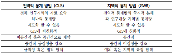
   • Cook's Distance can be calculated as \(D_i = \frac{r_i^2}{p} \times \left( \frac{h_{ii}}{1-h_{ii}}\right)\) Where \(\begin{align*} r_i = \text{Studentized residual}\\ h_{ii} = \text{Leverage} \\ p = \text{number of variables} \end{align*}\) —

     비교

     

---

Total algorithm

---

Application

• https://rpubs.com/zirumo07/463009

• https://www.emilyburchfield.org/courses/gsa/spatial_regression_lab

  Reference

• 지리적 가중회귀모형을 이용한 지역별 심정지 발생요인에 관한 연구
• 공간 자료를 이용한 대기오염이 순환기계 건강에 미치는 영향 분석
• Comparison of Ordinary Least Square Regression, Spatial Autoregression, and Geographically Weighted Regression for Modeling Forest Structural Attributes Using a Geographical Information System (GIS)/Remote Sensing (RS) Approach
• Lee, S.-I. Correlation and Spatial Autocorrelation. In Encyclopedia of GIS; Shekhar, S., Xiong, H., Zhou, X., Eds.; Springer International Publishing: Cham, Switzerland, 2015; pp. 1–8.
• Ren, T.; Long, Z.; Zhang, R.; Chen, Q. Moran’s I test of spatial panel data model—Based on bootstrap method. Econ. Model. 2014, 41, 9–14.